
Why Pacing Models?
If you're a private equity investor, you've probably asked this question more than once:
“How will my capital actually flow in and out over the life of a fund?”
While no model will give you a perfect forecast, having a solid one is crucial. A good pacing model helps you:
- Stay on top of liquidity needs
- Avoid overcommitment
- Align with your target allocations
- Better understand your risk profile
In this post, I’ll walk you through the two main types of pacing models and the most common forecasting methods used by industry professionals and vendors. This guide is based on research across the leading providers in the space.
Two Main Types of Pacing Models
✅ Deterministic Models
These models give you a single outcome based on a fixed set of assumptions. They’re useful for scenario modeling and sensitivity analysis.
- Pros: Clear, transparent, and fast to run
- Cons: No view into uncertainty or risk ranges
✅ Stochastic Models
These models generate a range of possible outcomes, each tied to probabilities or confidence intervals—often using Monte Carlo simulations.
- Pros: Ideal for stress testing and risk management
- Cons: More complex to implement and interpret
5 Applied Methods to Build a Pacing Model
1. Bootstrapping (Using Cash‑Flow Libraries)
You select a library of vintage‑matched funds with quarterly or annual cash‑flow sequences. Pick the peers closest to your size, vintage, and strategy—then stretch or scale those curves to reflect your fund’s expected tempo and commitment profile.
Both deterministic ("template‑based") and stochastic implementations exist, with the latter sampling real cash‑flow histories per each iteration.
✅ Gold standard for empirical pacing accuracy and proper J‑curve realization.
⚠️ Needs extensive, high‑quality, unbiased data and care to avoid sampling bias.
Optionally you can substitute peer groups to stress test alternative pacing patterns.
2. DPI & PICC Method
When full cash‑flow sequences aren’t available, benchmark curves for DPI (Distributions ÷ Paid‑In) or PICC (Paid‑In ÷ Commitment) can serve as a proxy. You back‑solve contributions and distributions to fit these benchmark ratios over time.
Works in both deterministic or stochastic mode depending on whether you use point estimates or sample from a curve distribution.
✅ Easier to access than full sequences—suitable for high‑level pacing insights.
⚠️ May oversimplify timing and ignores specific fund behavior nuance or structural variation.
3. Rules‑Based Approach
This relies on simple, deterministic formulas developed from historical research and simulations. A widely used rule is:
Annual Commitment Rate = Target Allocation % ÷ Pacing Divisor
The divisor is calibrated by asset class—e.g. buyout, venture, real estate, or infrastructure.
✅ Fast, transparent, minimal inputs; great for early budgeting and static allocation planning.
⚠️ No modeling of distributions, NAV evolution, timing, or stress testing. It’s essentially a static pacing shortcut.
4. Machine Learning
ML models (neural networks, LSTM/GRU, etc.) are trained on historical fund cash flows, macroeconomic indicators, and public markets data to predict future call and distribution patterns.
✅ Can detect subtle, non‑linear relationships and adapt to different macro regimes, potentially outperforming curve-based models.
⚠️ High complexity ("black box"), requires massive clean datasets and rigorous modeling discipline. Risk of overfitting or miscalibration.
5. Takahashi & Alexander Model (Yale Model)
Originating from work at Yale, this deterministic model uses a compact set of parameters—fund life, call rate, growth (IRR), yield, bow factor, and initial unfunded/NAV—to model calls, distributions, and NAV over time:
Calls[t] = Unfunded[t−1] × CallRate
Distributions[t] = NAV[t−1] × (1 + GrowthRate) × DistributionRate[t]
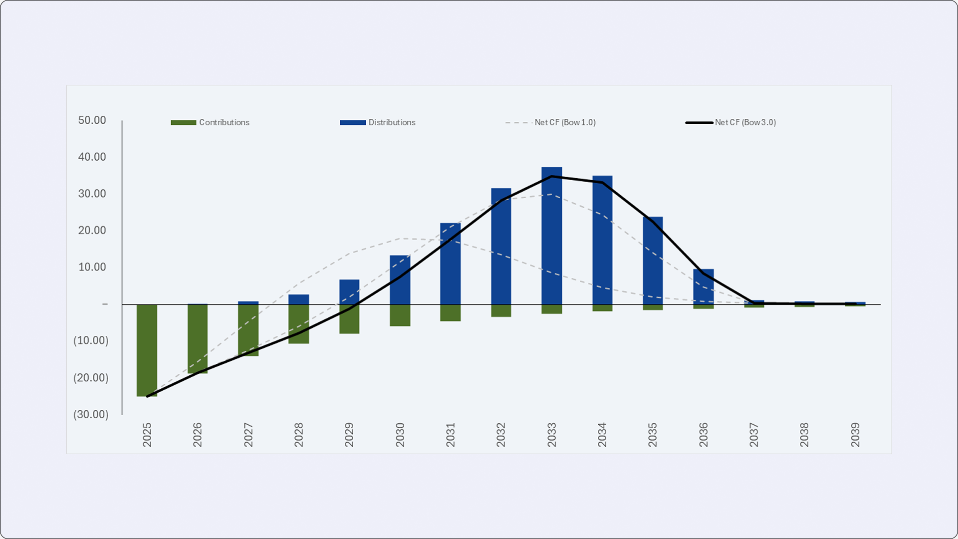
DistributionRate[t] = max(Yield, (Age / FundLife)^Bow)
NAV[t] = NAV[t−1] × (1 + GrowthRate) + Calls[t] − Distributions[t]
Variants exist that layer stochastic sampling on top of these formulas.
✅ Transparent, easy to explain, fast to calibrate and scenario-test, and flexible across asset types.
⚠️ Assumes static parameters and lacks timing risk modeling. Outputs should guide—not dictate—forecast decisions.
Choosing the right pacing model depends on your data availability, internal capabilities, and desired level of precision.